The Kernel Trick (An Intuitive Explanation)
What is this post about?
Although there are many good resources explaining the idea of the kernel trick out there, the majority is in my opinion quite convoluted (wink, wink). Here, I attempt to demistify the concept by pointing out several key features of The Kernel Trick, while still using the well-recognized example of a non-linear classification problem. It is an attempt at the most intuitive explanation of The Kernel Trick.
The starting point
To begin, let’s consider a toy example of hundred random points scattered on a 2D plate. The points closer to the center are of the blue type, while the points further away from the center are of the red type. If it helps, imagine it’s a plate with blueberries around the center and raspberries on the outside. What we would like to do is to make a model that can predict whether the point is blue (the berry is a blueberry) or red (the berry is raspberry) based on its $x$ and $y$ coordinates.
Since linear models are way better understood, simpler to build, and simpler to interpret, we would like to use a linear model to do this. What this entails is that we would simply like to draw a single straight line on our 2D plate that separates the blueberries from the raspberries as cleanly as possible.
Looking at the picture of our toy example below, this proves quite hard. What we would much rather do is draw a circle and classify the berries into those inside it and those outside of it. However, a circle is a non-linear separation boundry on our 2D plate, so bad luck for us… Or maybe not?
Code
import numpy as np
import matplotlib.pyplot as plt
from matplotlib.offsetbox import OffsetImage, AnnotationBbox
from mpl_toolkits import mplot3d
import pandas as pd

def main():
    # Seed
    np.random.seed(42)

    # Coordinates
    x = np.random.uniform(-2, 2, size = 100)
    y = np.random.uniform(-2, 2, size = 100)
    c = np.array(['dodgerblue' if zi <= 1 else 'red' for zi  in z])

    # Images
    bb_path = get_sample_data("blueberry.png")
    rb_path = get_sample_data("raspberry.png")

    # Plot
    fig, ax = plt.subplots(figsize = (7,7))
    imscatter(x[np.where(c == 'dodgerblue')], y[np.where(c == 'dodgerblue')],
    bb_path, zoom = 0.04, ax = ax)
    imscatter(x[np.where(c == 'red')], y[np.where(c == 'red')],
    rb_path, zoom = 0.06, ax = ax)
    ax.scatter(x, y)

    # Axes
    ax.set_yticks(np.linspace(-2, 2, 5))
    ax.set_xticks(np.linspace(-2, 2, 5))
    ax.set_ylabel('y')
    ax.set_xlabel('x')

    # Center lines
    ax.axvline(0, 0, linestyle = '--', lw = 1, color = 'black', alpha = 0.5)
    ax.axhline(0, 0, linestyle = '--', lw = 1, color = 'black', alpha = 0.5)

    # Circles
    ax.add_patch(plt.Circle((0, 0), 0.5, fill = 'dodgerblue', linestyle = '--', lw = 1, alpha = 0.3))
    ax.add_patch(plt.Circle((0, 0), 1, fill = 'dodgerblue', linestyle = '--', lw = 1, alpha = 0.2))
    ax.add_patch(plt.Circle((0, 0), 1.5, fill = 'dodgerblue', linestyle = '--', lw = 1, alpha = 0.1))

    plt.show()

def imscatter(x, y, image, ax = None, zoom = 1):
    if ax is None:
        ax = plt.gca()
    try:
        image = plt.imread(image)
    except TypeError:
        pass
    im = OffsetImage(image, zoom = zoom)
    x, y = np.atleast_1d(x, y)
    artists = []
    for x0, y0 in zip(x, y):
        ab = AnnotationBbox(im, (x0, y0), xycoords = 'data', frameon = False)
        artists.append(ax.add_artist(ab))
    ax.update_datalim(np.column_stack([x, y]))
    ax.autoscale()
    return artists

main()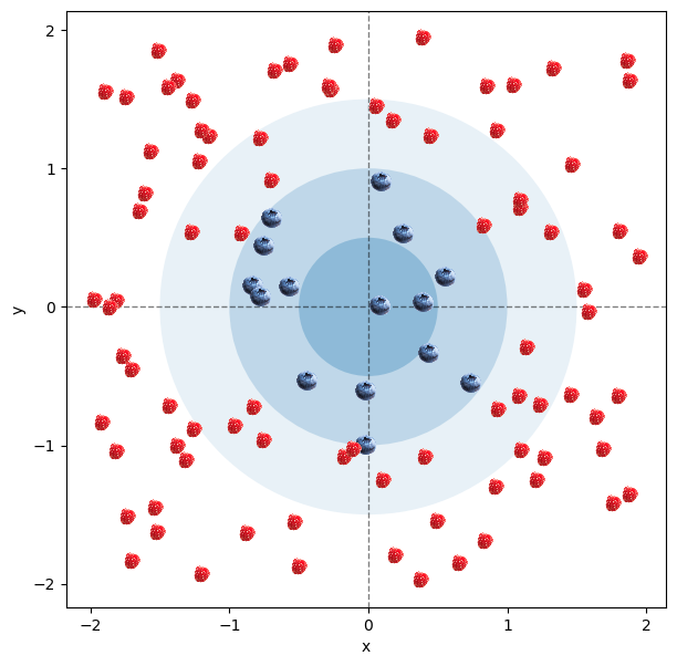
What we want
If we think about the problem carefully, one idea that we might come up with is to add another feature that describes some additonal characteristic of each individual berry. We would like this feature to be such that it makes it easier to separate the two groups. Under this setup, every point would be described by three coordinates $(x, y, z)$ instead of just two $(x, y)$.
What would be a good $z$ that would make our problem much easier - that is, linearly separable? A good candidate $z$ is $z = x^2 + y^2$. This is because if a point is close to the center at $(0,0)$, $z$ will be small. Conversely, if the point is far away from the center, e.g. a point at $(-1.5, 1)$, $z$ will be large.
Thus calculating $z$ for each point and plotting the points in 3D gives us the picture below. As expected, the blue points are much lower than the red points. Moreover, it looks like we can separate the two classes with a 2D plane, which means the problem became linearly seperable. Nice!
Wonderful, we solved it, job done. Or?
Code
# Calculate the new feature
z = x**2 + y**2

# Plot the points in 3D
fig = plt.figure(figsize = (plt.figaspect(0.4)))

# Side view
ax = fig.add_subplot(1, 2, 1, projection = '3d')
ax.set_title("Side View", y = 1)
ax.scatter3D(x, y, z, c = c)
ax.view_init(elev = 10, azim = 135)
ax.grid(False)
# Axes
ax.xaxis.pane.set_edgecolor('black')
ax.set_xlabel('x')
ax.set_ylabel('y')
ax.zaxis.set_rotate_label(False)
ax.set_zlabel('$x^2+y^2$', rotation = 0)
ax.yaxis.pane.set_edgecolor('black')
ax.zaxis.pane.set_edgecolor('black')
ax.xaxis.pane.fill = False
ax.yaxis.pane.fill = False
ax.zaxis.pane.fill = False

# Top view
ax = fig.add_subplot(1, 2, 2, projection = '3d')
ax.set_title("Top View", y = 1)
ax.scatter3D(x, y, z, c = c)
ax.view_init(elev = 90, azim = -90)
ax.grid(False)
# Axes
ax.set_xlabel('x')
ax.set_ylabel('y')
ax.zaxis.set_ticks([])
ax.xaxis.pane.set_edgecolor(None)
ax.yaxis.pane.set_edgecolor(None)
ax.zaxis.pane.set_edgecolor(None)
ax.xaxis.pane.fill = False
ax.yaxis.pane.fill = False
ax.zaxis.pane.fill = False

plt.show()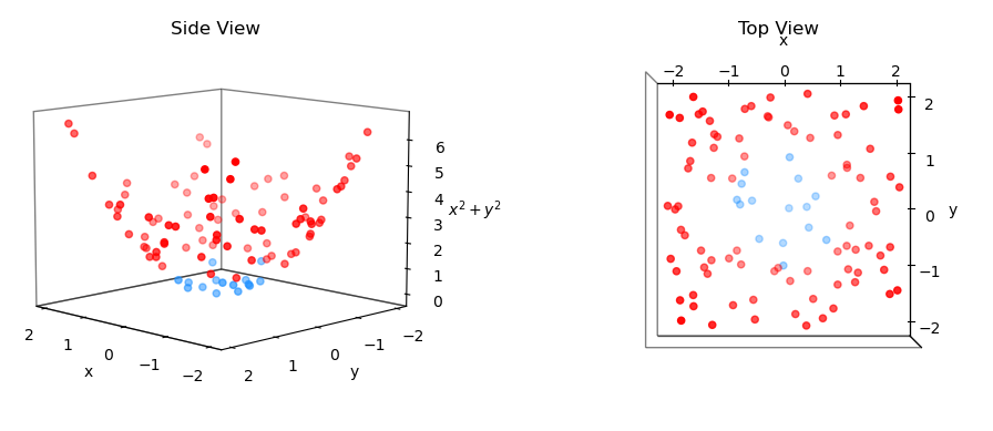
What we get
Well, not so fast, we haven’t used the kernel trick yet!
So here it is, The Kernel Trick:
Looking again at our toy example, what we are really interested in is NOT the exact $z$ coordinate of each point. Rather we want to know how each point relates to each other in the new 3-dimensional space. How similar or distinct the points are, and what is the (dis)similarity threshold at which we say this point right here is a blueberry, and this other point over there is raspberry. The kernel trick exploits exactly this idea.
Instead of computing the actual values of the new coordinates for each point, a kernel function computes some distance measure between all pairs of points in some higher-dimensional space. In our toy example, this would mean that the kernel trick would never produce the 3-dimensional pictures above explicitly! All the kernel function would give us are the 3D (dis)similarities between the points, but never their actual 3D coordinates. I’ve repeated this twice, I know, but I think this is what most explanations are missing. This idea of only computing the pseudo-distances is the actual “trick” in the kernel trick. But if you still don’t see why we call it a “trick”, let’s disect it a little further.
In the above 3D picture, computing (some) distance measure between two points $i$ and $j$ would require us to consider all 3 of their coordinates, $(x_i, \; y_i, \; z_i)$ and $(x_j, \; y_j, \; z_j)$. Why kernel trick is called a “trick”, is that this distance measure is computable without ever having to explicitly know or compute all of these coordinates. Since that is the case, the kernel trick will never be able to tell us what the exact position of the point $i$ or $j$ in 3D is, since it will never compute the new coordinates. However, we couldn’t care less, since all we want to know is how $i$ relates to $j$ in 3D, and the kernel trick can readily provide us with that answer.
How it does so, and this is the second important property of the kernel trick that’s key here, is by defining the distances or (dis)similarities as dot products between the vectors in the higher-dimensional space. In our examples above, the (dis)similarity between points $i$ and $j$ would be computed as $i \cdot j$ or $(x_i \quad y_i \quad x_i^2+y_i^2)(x_j \quad y_j \quad x_j^2+y_j^2)^T$. With this definition, it is (sometimes) possible to compute $i \cdot j$ in 3D by applying some kernel function $k$ to their inner product $k(i \cdot j)$ in 2D. Which is exactly the “trick” here! We define a kernel function $k$ that computes the dot products in 3D, but it does so by only ever considering the coordinates in 2D, never in 3D (the higher dimension).
So to repeat, the magic of the kernel trick comes from three of its key properties:
- It only considers the distances between the points in some higher-dimensional space
- It defines these distances as inner products of their coordinates in this higher-dimensional space
- It computes these distances as some function $k$ on the inner products of the coordinates in our original lower-dimensional space
Applying the kernel trick
Now when we understand what the “trick” in the kernel trick stands for, let us use it to implicitly re-create our 3D mapping above.
What we would like to do is to apply a kernel function that’s equivalent to computing
\[\begin{pmatrix}x_i \quad y_i \quad x_i^2 + y_i^2\end{pmatrix}\cdot\begin{pmatrix}x_j \\ y_j \\ x_j^2 + y_j^2\end{pmatrix}\]for all pairs of points $i$ and $j$ while only considering their known coordinates $(x_i, \; y_i)$ and $(x_j, \; y_j)$. Expanding the above defined dot product we get,
\[x_ix_j + y_iy_j + (x_i^2 + y_i^2)(x_j^2 + y_j^2).\]With an eye trained for spotting vector operations, we notice that this can be rewritten in a vector form as:
where the final equality is our kernel function $k(i,j) = i\cdot j + \vert\vert i\vert\vert ^2\vert\vert j\vert\vert^2$! Magic!
But did you notice what we just did?! We applied the 3 key properties of the kernel trick step by step. We decided to consider the distances between $i$ and $j$. We defined these distances as the inner products in the 3D space. And we computed a function that takes in 2D coordinates of $i$ and $j$, and spits out the inner product of their 3D representations. No magic, just smart application of linear algebra and a good deal of inventivness!
Bellow I apply this newly acquired knowledge in code, and as in the visual example above, the results below show us that using the kernel trick, the average inner product distances between two blueberies are the smallest, followed by the distances between a blueberry and a raspberry, further followed by the distances between two raspberries. Quite nice, huh? So essentially the kernel trick gave us a new perspective on the old problem. Before, we were looking at blue and red points in 3D and we could see that we can probably separate them with some well chosen 2D plane stuck inside the cone that they created. With the kernel trick, we have the information about all the pair-wise dot product distances between the points, and we can use them to again quite easily separate the blue points from the red ones. Same problem, different approach, new insight, equivalent solution. Nice!
# Define our kernel
def circleKernel(x, y):
    return np.dot(x,y) + np.dot(x,x)*np.dot(y,y)

# Apply our kernel on the 2D feature matrix X with dimensions (100 x 2)
X = list(zip(x,y))
kernelTrick = np.array([[circleKernel(x, y) for x in X] for y in X])

# Check the output dimensions of the "Kernel Trick"
print(f"The kernel matrix has a shape: {kernelTrick.shape}")
The kernel matrix has a shape: (100, 100)
# Transform the kernel matrix into a long-format list
longKernel = [[i, j, kernelTrick[i][j]] for i in range(len(kernelTrick)) for j in range(i, len(kernelTrick[i]))]

# Sort the kernel distances from the smallest to the longest
longKernel.sort(key = lambda x: x[2])
for i in longKernel:
    if c[i[0]] == "dodgerblue":
        i.append("blue")
    else:
        i.append("red")
    if c[i[1]] == "dodgerblue":
        i.append("blue")
    else:
        i.append("red")

# Show the 15 shortest distances
longKernel = pd.DataFrame(longKernel, columns = ['Point i', 'Point j', 'Kernel Distance', 'Color i', 'Color j'])
print("15 shortest kernel distances:\n" + "-" * 62)
print(longKernel.head(15))
print("-" * 62)

# Show the 15 longest distances
print("\n15 longest kernel distances:\n" + "-" * 62)
print(longKernel.tail(15))
print("-" * 62)

# Compute the average distances between the blue and red points
blues = longKernel['Kernel Distance'].loc[(longKernel['Color i'] == 'blue') & (longKernel['Color j'] == 'blue')].mean()
reds = longKernel['Kernel Distance'].loc[(longKernel['Color i'] == 'red') & (longKernel['Color j'] == 'red')].mean()
mix = longKernel['Kernel Distance'].loc[longKernel['Color i'] != longKernel['Color j']].mean()

# Show the average kernel distance
print(f'\nAverage distance for 2 blue points: {blues}')
print(f'Average distance for 2 mixed points: {mix}')
print(f'Average distance for 2 red points: {reds}')
15 shortest kernel distances:
--------------------------------------------------------------
    Point i  Point j  Kernel Distance Color i Color j
0        30       85        -0.247890    blue    blue
1        95       96        -0.246702    blue    blue
2        30       46        -0.245391    blue    blue
3        30       61        -0.239791    blue     red
4        60       93        -0.226513    blue    blue
5        30       59        -0.213364    blue     red
6        25       63        -0.211831     red    blue
7         3       19        -0.210847    blue    blue
8         3       36        -0.209118    blue    blue
9        38       63        -0.207110    blue    blue
10       89       93        -0.206464     red    blue
11       24       93        -0.205008     red    blue
12       93       95        -0.202019    blue    blue
13        3       77        -0.200195    blue     red
14        3        6        -0.199416    blue     red
--------------------------------------------------------------

15 longest kernel distances:
--------------------------------------------------------------
      Point i  Point j  Kernel Distance Color i Color j
5035       68       90        36.707447     red     red
5036       12       34        36.726950     red     red
5037       83       98        37.611562     red     red
5038       68       98        38.014602     red     red
5039       68       71        38.154232     red     red
5040       34       40        38.174184     red     red
5041       40       40        38.281834     red     red
5042       34       98        38.860370     red     red
5043       32       68        39.230553     red     red
5044       40       98        39.984242     red     red
5045       98       98        42.013085     red     red
5046       50       50        44.573723     red     red
5047       68       68        45.587152     red     red
5048       34       50        47.326797     red     red
5049       34       34        50.269614     red     red
--------------------------------------------------------------

Average distance for 2 blue points: 0.3330975286504516
Average distance for 2 mixed points: 1.7035140320881144
Average distance for 2 red points: 10.140681935021039
Concluding thoughts
I hope this explanation made the idea of the kernel trick quite a lot clearer. It’s a pretty neat, but also quite an abstract idea so I totally understand if you haven’t yet fully wrapped your head around it. Took me a while, and I am sure I will need to remind myself of what the kernel trick actually is in the future again. But for now, happy kerneling :)