Matrix Tree Theorem - Actually Explained
Intro
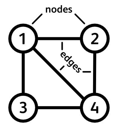
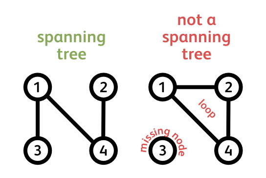
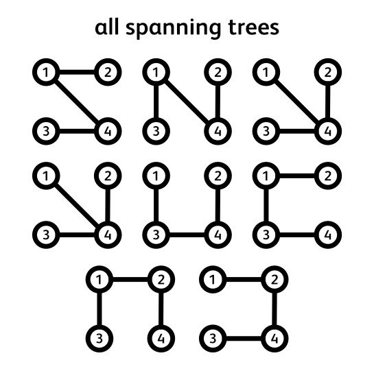
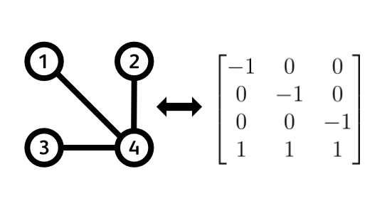
This is a graph. It consists of nodes connected by edges. A spanning tree, is a subgraph that connects all the nodes without forming any loops. In this graph we can count 8 such trees. But what if we are interested in a much larger graph? How many trees does it contain? Clearly counting them by hand isn’t feasible anymore. In fact, as the graph grows in the number of nodes, the number of trees may grow exponentially, so counting them by hand would literally take you a lifetime. Is there then a mathematical shortcut for counting the number of trees in a graph? Turns out there is, and a very fascinating one, here’s how it works:
Matrix Tree Theorem in a Nutshell
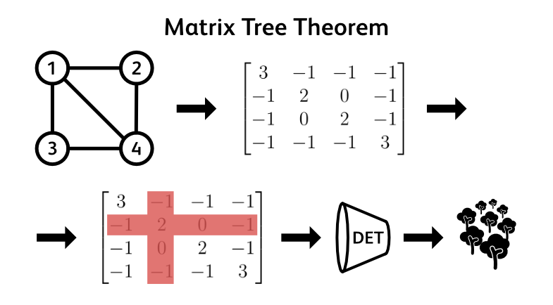
Every graph can be represented in terms of its nodes and edges. If we put these nodes and edges into a neat table we get a matrix representation of a graph. There are several such representations but the one we are interested in is called the Laplacian matrix. Here’s how it looks.
\[L = \begin{bmatrix} 3 & -1 & -1 & -1 \\ -1 & 2 & 0 & -1 \\ -1 & 0 & 2 & -1 \\ -1 & -1 & -1 & 3 \\ \end{bmatrix}\]In our case, it has 4 rows and 4 columns, one for each node in our graph. On the diagonal we write the number of edges that each node has. In our case it’s 3, 2, 2, and 3. The rest of the entries in the table are either 0s or -1s. You can think of each off-diagonal entry as a connection between the node in its row and a node in its column. If our graph has an edge between these two nodes, we write -1, if it doesn’t we write 0. If we do it correctly, every row and every column should sum to 0. For example the 3rd column contains -1 + 0 + 2 - 1 which sums to 0. Just like all other rows and columns. You can check it for yourself.
Now comes the fun part. To find the number of spanning trees of our original graph we need to delete one row and one column with the same index. For example, let’s delete the second column and the second row. We end up with a smaller matrix like this one.
\[L_{2,2} = \begin{bmatrix} 3 & -1 & -1 \\ -1 & 2 & -1 \\ -1 & -1 & 3 \\ \end{bmatrix}\]For any square matrix there exists a function that maps its contents to a real number: the determinant. We’ll revise some of its properties in a minute but for now all you need to remember is that it is a well defined algorithm that takes any square matrix and outputs a number. Well, running our reduced matrix through this algorithm gives us exactly what we are after: the number of spanning trees in our graph! For this graph, that’s 8.
Let that sink in… The determinant of a Laplacian with one of its rows and columns deleted gives us the number of spanning trees in the graph. What? How? Are you kidding me? If that’s what you are thinking, then welcome to the club. That was my reaction as well. How is this even possible? Worry not, it’s quite beautiful. We’ll take it step-by-step and by the end of this journey you should be able to see through the opaqueness of this black magic.
Gustav Kirchhoff
To begin this journey let us start with introducing Gustav Kirchhoff. Born in 1824 Prussia, Kirchhoff grew up to be a theoretical physicist who is today most well known for his work on electrical circuits. He published his fundamental laws of electrical circuits in 1845 while still an undergraduate. To put things in perspective, Michael Faraday discovered how electromagnetic generators work in 1831 and Thomas Edison patented the world’s first lightbulb more than 40 years later, in 1878. So we can call Kirchhoff somewhat of a futurist.
In his second paper, in 1847, a 21 year old Kirchhoff set out to proof two new theorems regarding electrical circuits. His setup included $n$ wires connected in an arbitrary fashion, all plugged into an electric generator. His main question was: Given the generator’s power output, how can I calculate the currents flowing through the wires? It is this paper to which the discovery of Kirchhoff’s Matrix Tree Theorem (MTT) is attributed. As you can see, the discovery of MTT is kind of an accident of history. Kirchhoff never really set out to calculate the number of spanning trees in a graph. It just happened to be that a randomly connected circuit of wires can be represented as a graph and that Kirchhoff’s question boiled down to counting the spanning trees of this graph. In fact, there’s some controversy regarding the attribution of the MTT as Kirchhoff never explicitly proves it in his paper. But we will, and unlike Kirchhoff, we will set out to do so with the sole purpose of understanding how it works, without electrical circuits getting in our way.
Graphs meet Linear Algebra
As we have already seen, graphs can be represented as matrices. We started by looking at how to translate a graph into its Laplacian matrix but there are more fundamental matrix-graph representations than the Laplacian. To understand the black magic of MTT we’ll need one more matrix representation of a graph:
The Incidence Matrix: $E$
Denoting the total number of nodes in our graph with little $n$ and the total number of edges with a little $m$, the incidence matrix consists of $n$ rows and $m$ columns. $n$ rows, one for each one of the nodes, and $m$ columns, one for each one of the edges. In its simplest form, each column represents an edge, containing exactly two 1s and $(n-2)$ 0s. As you might have guessed, the 1s are placed on the rows that the edge connects together and the 0s on the remaining entries in that column.
I say in its simplest from because this form represents an undirected graph. A graph where the edges are two-way streets. But, there also exist directed graphs, where the edges are one-way streets, or arrows. And in that case, each column of the incidence matrix includes a single -1 entry, a single +1 entry and again $(n-2)$ 0s. The -1 is placed on the row from which the edge (arrow) leaves and the 1 on the row to which the edge (arrow) arrives. Although the graphs we are concerned with are undirected, the two-way street version, to understand how MTT works we will use the one-way street/arrow version of the incidence matrix. To do so, we will just change each first 1 in a column to a -1 and continue as if we were still dealing with an undirected graph.
\[E = \begin{bmatrix} -1 & -1 & -1 & 0 & 0 \\ 1 & 0 & 0 & -1 & 0 \\ 0 & 1 & 0 & 0 & -1 \\ 0 & 0 & 1 & 1 & 1 \\ \end{bmatrix}\]Why did we do that last little trick? Well, it turns out that by doing so, this neat little formula emerges:
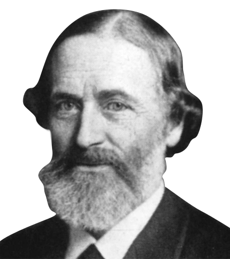
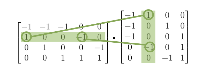
\[L = EE^T\]Yes, multiplying the Incidence matrix with its transpose gives us the Laplacian matrix. But this only works when the incidence matrix is oriented. We can quickly persuade ourselves that this works by looking at what happens when we want to calculate some on-diagonal and some off-diagonal entries of the Laplacian matrix $L$. For the diagonal entry, the dot product just results in multiplying all -1s with -1s and all 1s with 1s, so the result is the total number of edges adjacent to that particular node of the graph.
For the off-diagonal entry, the $i$-th row of $E$ contains 1s or -1s on all the positions where the node $i$ is connected to some other node $k$. These 1s and -1s are essentially “edge indicators” for that particular node $i$. They indicate all the half-edges that are connected to the node $i$. The same is true for the $j$-th column of $E^T$, but for some other node $j$ ($i$ $\neq$ $j$). Thus if we take the dot product of these two vectors, the result will be a 0, unless there is an edge between the nodes $i$ and $j$, and thus each vector has one of the corresponding “edge indicators”. If that’s the case, the result will be a -1, because each edge in an oriented incidence matrix consists of a 1 and a -1. Thus one of the nodes that this edge connects will have a 1 as its “edge indicator”, while the other will have a -1.
If this is clear, then it shouldn’t be so surprising that the following also holds:
\[L_{ii} = E_i{E^T}_i\]The $i$ sub-scripts here stand for the row or column that’s deleted from the original matrix. So $L_{ii}$ is the Laplacian with its $i$-th row and $i$-th column deleted, while $E_i$ is the incidence matrix with its $i$-th row deleted. That covered, we can move onto some fun facts about the determinant function.
The Peculiarities of the Determinant Function
So to stay on top of our mission, let’s recap what we are doing. To get the number of spanning trees in a graph, we take the graph’s Laplacian matrix, delete a row and a column with the same index, and then compute the determinant of this reduced matrix. Why do we perform the deletion step? Why can’t we just compute the determinant straight away?
As we have already seen at the very beginning, the sums across all rows and all columns of the Laplacian yield the zero vector. This means that the columns (and rows) are linearly dependent and thus the determinant is 0.
\[\begin{equation} \left[ \begin{array}{cccc|c} 3 & -1 & -1 & -1 & + \\ -1 & 2 & 0 & -1 & + \\ -1 & 0 & 2 & -1 & + \\ -1 & -1 & -1 & 3 & + \\ \hline 0 & 0 & 0 & 0 & \end{array} \right] \end{equation}\]This is just a basic fact taught in any introductory Linear Algebra course. When the columns are linearly dependent, the determinant is 0. In the following few lines I will not attempt to proof or derive from scratch other properties of the determinant function, that’s a quest for an entirely different deep dive, but I will list some basic properties of the determinant which will come useful in understanding the black magic we set out to uncover. Here are the properties of the determinant function that will come handy:
- Determinant of a matrix product equals the product of determinants: $\text{det}(AB)=\text{det}(A)\text{det}(B)$
- Determinant of a transpose is the same as the determinant of the original matrix: $\text{det}(A) = \text{det}(A^T)$
- An $n \times n$ matrix with less than $n$ linear independent columns will always have determinant = 0
Trees meet Matrices and Determinants
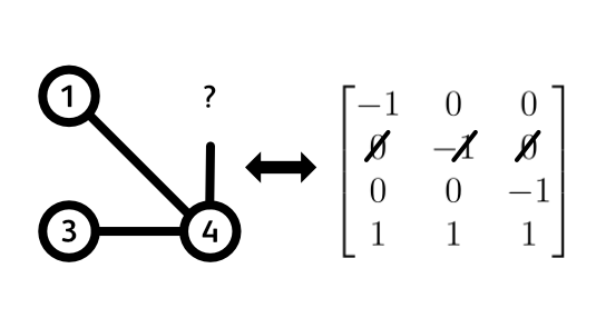
Given what we now know about determinants, let’s see whether there’s any connection we can make between them and spanning trees. A spanning tree on $n$ nodes has exactly $n - 1$ edges. This is a fixed constraint. If it had more, there would be at least one loop in the graph, if it had less, there would be at least one node left out. So it must have exactly $n - 1$ edges. Thus an incidence matrix of a spanning tree is a matrix with $n$ rows (nodes) and $n - 1$ columns (edges). Since it is not a square matrix, it doesn’t have a determinant. Hmm, that’s a bit troublesome.
But what if we deleted one of the rows to get an ($n - 1$) by ($n - 1$) sub-matrix? You might protest to this with something like: “But then it’s not a true incidence matrix of a spanning tree!”. You are absolutely right, but let’s entertain this crazy idea for a moment. Deleting one of the rows is essentially equivalent to deleting one of the nodes from our graph. What will happen to its edges? Well, it is as if we cut them in half. Because every column of the incidence matrix represents an edge, deleting a single row will delete one half (a 1 or a -1) of each edge that was incident to that row (node). However, we still have the other half of the edge. So my point here is this: deleting a row from an incidence matrix doesn’t cause any information loss about the actual structure of the graph. This is because all the edges that were not incident to the deleted node are still intact, and the incident edges were just cut in half. Since we are left with all the remaining nodes, all the remaining edges, and some half-edges, we can revert to our original graph whenever we want. We just add back in a node, and only reconstruct the half-edges without touching anything else. Hope this is persuasive enough.
Let us then continue. We deleted a random row, so we are left with a square ($n - 1$) by ($n - 1$) sub-matrix that has some determinant (since it’s a square matrix). What’s the value of this determinant? Is it always 0? Always non-zero? Always some specific value? To get down to this, let’s begin by determining (pun intended) the rank of this submatrix. That is, how many linearly independent rows does it have?
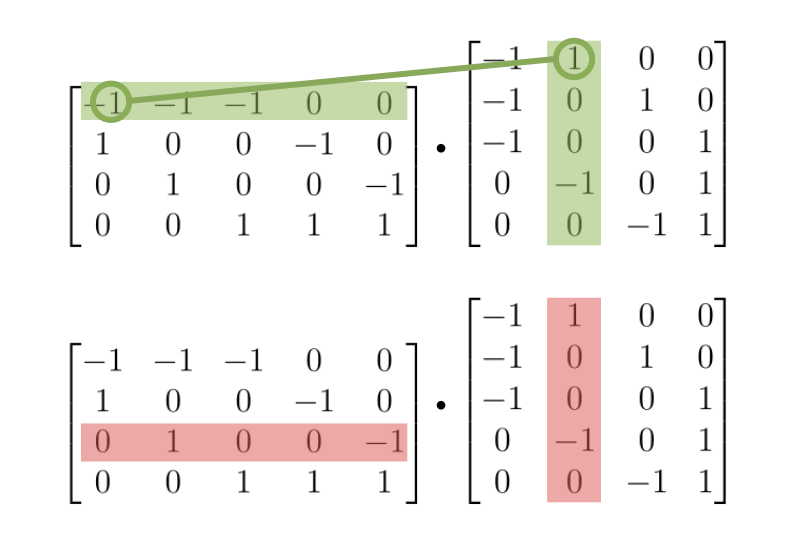
Because this is at the core of understanding the MTT, let us go through a little proof. We start with our original incidence matrix and find its rank. Based on that, it will be easy to determine a rank of a sub-matrix obtained by a deletion of a single row. So, since every column of the original incidence matrix has exactly a single +1 entry and a single -1 entry, the sum of all the rows gets us the 0 vector.
\[\begin{equation} E_{tree} = \left[ \begin{array}{ccccc|c} -1 & 0 & 0 & + \\ 0 & -1 & 0 & + \\ 0 & 0 & -1 & + \\ 1 & 1 & 1 & + \\ \hline 0 & 0 & 0 & \end{array} \right] \end{equation}\]Therefore the rows are linearly dependent and the rank is for sure $\leq n$. Alright, is the rank $n - 1$ then? Well, let’s see if there is some other linear combination of rows that yields the zero vector. If there is, then the rank is even less than $n - 1$, but if there isn’t, the rank is exactly $n - 1$. If we denote an arbitrary row of our matrix as $R_j$, a linear combination we are after is $\sum_{j=1}^n c_jR_j = 0$, where $c_j$ is a scalar coefficient we multiply each row by, and the sum must have at least one non-zero $c_j$. The linear combination we already have is the one where $c_j = 1$ for all $j$. Let’s now try and construct a different one. Say that for some arbitrary row $R_r$ the coefficient $c_r \neq 0$. This will affect all the non-zero entries of $R_r$ and for every non-zero entry of $R_r$, there is a non-zero entry with the opposite sign in some other row $R_{s}$. In order for our linear combination to sum to 0, the coefficients $c_{s}$ of all the other rows $R_{s}$ must therefore be the same as $c_r$. But because we are dealing with a connected graph (a spanning tree), every node (row) is reachable from every other node (row) and thus all $c_j$ must be equal for our linear combination to hold. This thus yields that the only possible linear combination is $c \left(\sum_{j=1}^n R_j\right) = 0$, which is precisely our first linear combination - a sum of all rows, all multiplied with the same coefficient, we just chose $c=1$. Since, we have shown there is just this one way of combining the rows to get the zero vector, we have shown that the rank of an oriented incidence matrix corresponding to a fully connected graph is $n-1$. Noice!
What does this mean for our square sub-matrix obtained by a deletion of a single row? Well, there are $n$ rows and $n-1$ of them are linearly independent. Thus if we delete one row, we will end up with some $n-1$ linearly independent rows. Conclusion: the sub-matrix obtained by a row deletion has full rank: $n-1$ linearly independent rows while its size is $(n-1)\times(n-1)$. Consequence for the determinant? The determinant is certainly NOT 0. Good, what is it then? In the following paragraph I will try and persuade you that it is either +1 or -1. But for that we will use one more concept called Total Unimodularity.
Total Unimodularity is a property of matrices leveraged in the field of linear optimization. It states that matrix $A$ of size $m$ by $n$ is Totally Unimodular if all its square sub-matrices (of any size) have determinants equal to 0, +1, or -1. In the field of linear optimization, this property is leveraged to guarantee integer solutions to some specific problems, but that’s yet another topic for a whole different deep dive. How will we use it here? Well, those specific problems I just mentioned all use incidence matrices, just as we are. And the oriented incidence matrices, like ours, have been proven to always be Totally Unimodular. What does this mean for us? Well, if the incidence matrix of a spanning tree is Totally Unimodular, the ($n - 1$) by ($n - 1$) sub-matrix we obtain by deleting an arbitrary row has determinant of 0, +1, or -1. But we have just shown that the rank of this sub-matrix is $n - 1$ and thus it cannot have a determinant of 0. It’s full rank. Therefore, it must have a determinant equal to either +1 or -1. And that’s it, we’ve got it! The answer to our question of relating trees to determinants is that an incidence matrix of a valid spanning tree with one of its rows deleted will always, I repeat always, have a determinant of +1 or -1!
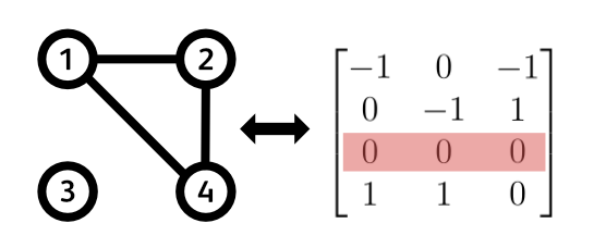
Before we begin the celebrations, an important question is: Can we distinguish a valid spanning tree from a non-valid one? Or put differently: Can we tell apart a random assemblance of $n - 1$ edges on $n$ nodes from a spanning tree? Answer is, we can! If $n -1$ edges don’t form a spanning tree, it means that some node is necessarily left out (and there is some loop). Therefore an incidence matrix of such a graph will have at least one row full of zeros. This means that the rank of this matrix is strictly less than $n - 1$ and therefore the rank of a sub-matrix with one deleted row is also strictly less than $n - 1$. As a consequence, the determinant of this sub-matrix must be 0 because its $n - 1$ rows are still linearly dependent in some way.
And there it is! This is the time for pausing and pondering what we have just went through. We found a link between spanning trees and determinants that distinguishes between valid spanning trees and a random assemblance of $n - 1$ edges. A spanning tree will yield a determinant of +1 or -1, while random assemblance of edges will always result in a determinant of 0. Let’s now leverage this property, and close up the case of how the black magic of Matrix Tree Theorem works.
The Puzzle Solves Itself
The puzzle solves itself… almost. Let’s begin the final chapter of our quest by recapping what we have already learned:
- the Laplacian matrix is a product of incidence matrices: $L = EE^T$
- this also holds if we delete a column/row: $L_{ii} = E_i{E^T}_i$
- an incidence matrix of a spanning tree with a single deleted row has determinant = +1/-1
- an incidence matrix of a $n - 1$ edges that don’t from a spanning tree with a single deleted row has determinant = 0
- and of course, the determinant of a Laplacian with one of its rows and columns deleted gives us the total number of spanning trees in a graph
That’s a lot that we know already. The final quest is just putting it all together. And for that we will need the final piece of the puzzle: Cauchy-Binet Theorem. The Cauchy-Binet theorem is a generalization of $\text{det}(AB)=\text{det}(A)\text{det}(B)$ for the case where $A$ and $B$ are not square matrices. If this rings a bell, that’s because that’s exactly our case. The incidence matrix $E_i$ is not a square matrix in general (in our little example it was just by accident) but $E_i{E^T}_i$ is square, so the Cauchy-Binet Theorem tells us how the determinants of $E_i{E^T}_i$, $E_i$, and ${E^T}_i$ are related. It is stated as follows:
This is very similar to the original rule with square matrices, but we added a sum over the set $S$. What is this set? The matrix $E_i$ is the incidence matrix of our entire graph with one of its rows (nodes) deleted, so its size is $(n - 1)$ by $m$, where $n$ is the number of nodes and $m$ is the number of edges. Because we are dealing with fully connected graphs, we only consider the case where there are at least as many edges as nodes, $m \geq n$. The set $S$ then consists of all the ways one can choose $n - 1$ edges from all of the $m$ available edges. The size of this set is therefore $\binom{n-1}{m}$: $(n-1)$ choose $m$. Picking some assemblance of $n-1$ edges from this set, the matrix $E_{i_S}$ is an $(n - 1)$ by $(n - 1)$ matrix whose $n - 1$ columns correspond to the edges we picked from the set $S$. So what the Cauchy-Binet theorem states is that the determinant of $L_{ii}$ is the sum of squared determinants of all possible combinations of $n-1$ edges from our graph.
If that last sentence gave you an ahaaa moment, then you’ve cracked the code. Indeed, the determinant of the Laplacian with one of its rows and columns deleted can be computed as a sum of squared determinants of the incidence matrices that correspond to all the ways we can pick $n-1$ edges from our graph. That’s a mouthful but let’s break it down. As we have shown before, if $n-1$ edges do NOT form a spanning tree, the determinant of their reduced incidence matrix will be 0. This means, all of these non-spanning trees will not contribute anything to the overall sum. However, if the $n-1$ edges DO form a spanning tree, the determinant of their reduced incidence matrix will be +1 or -1. Squaring it always yields 1, and thus every spanning tree adds exactly 1 to the overall sum. And that’s it, that’s all there’s to it. This is how the Matrix Tree Theorem works. It all stands on the Cauchy-Binet theorem and the distinguishing factor between valid and non-valid spanning trees and their determinants. Beautiful. If you ask me. I hope you agree.