Minimization by Majorization
What is this post about?
What follows is an intuitive explanation of Minimization by Majorization. I use multiple-linear regression as a concrete example to show the method and the derivation of the majorizing function. The content is based on the first lecture of Supervised Machine Learning course given at Erasmus University Rotterdam by P. Groenen.
Introduction
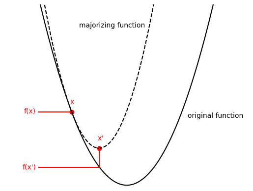
Minimization by majorization is one of many ways to find a minimum of a function. Given a function $f(x)$ we want to minimize, MM does so by defining a majorizing function $g(x, y$), that is adjacent to $f(x)$ at exactly one point, and larger than $f(x)$ everywhere else. If $g(x, y)$ fulfills these conditions, it can be used as a guide to traverse our original function $f(x)$ to find parameters $x$ that minimize it. Below you can see a toy example. Obviously, our original function here is very simple and we could have found its minimum directly, however, for explaining the concept, this toy example should serve us well. Given that $g(x, y)$ is simple, finding $(x, y)$ that locate its minimum is also assumed to be simple. Thus, as seen in the toy example, given our current $g(x, y)$, our next $x’$ will be the point defined by the minimum of $g(x, y)$ projected onto $f(x)$. This is shown in red in our example. Now you can imagine that at this new point $x’$, we can again define a new majorizing function $g(x’, y)$ and perform an equivalent step towards a more optimal point $x’’$. And so we do this until we find the optimal $\hat{x}$, which we can say happens when the relative difference between $x’$ and $x’’$ is smaller than some small $\epsilon$. The smaller the $\epsilon$ the better the precision but also the longer the convergence. Let’s now make this more concrete and look at how this would look like in a case of linear regression.
Linear Regression Equation
In matrix form, the linear regression is the well-known $\mathbf{X}\boldsymbol{\beta} = \boldsymbol{y}$. To find the vector of regression coefficients that are the most optimal, we minimize the sum of squared residuals $SSR = (\mathbf{X}\boldsymbol{b} - \boldsymbol{y})^T(\mathbf{X}\boldsymbol{b} - \boldsymbol{y}) = \boldsymbol{b}^T\mathbf{X}^T\mathbf{X}\boldsymbol{b} - 2\boldsymbol{b}^T\mathbf{X}^T\boldsymbol{y} + \boldsymbol{y}^T\boldsymbol{y}$ and obtain the closed form solution $\boldsymbol{b} = (\mathbf{X}^T\mathbf{X})^{-1}\mathbf{X}^T\boldsymbol{y}$. This should all be business as usual, but what would we do if we wanted to find the best fitting regression coefficients using the MM approach?
We have to again start from our point of departure, the $SSR$. By parametrizing $SSR$ with the $\boldsymbol{b}$ coefficients, we obtain our function of interest $f(x) = SSR(\boldsymbol{b})$. The leading term defining the shape of $SSR(\boldsymbol{b})$ is $\boldsymbol{b}^T\mathbf{X}^T\mathbf{X}\boldsymbol{b}$, hence we need to find some function $g(\boldsymbol{b}, \boldsymbol{b_0})$ that is larger and at most equal to $\boldsymbol{b}^T\mathbf{X}^T\mathbf{X}\boldsymbol{b}$, since that’s the definition of a majorizing function. How do we do this?
We look to find some inequality that on LHS has our term of interest plus some other terms, and on the RHS has a 0. This will let us shuffle the terms from left to right, hopefully obtaining an inequality with $\boldsymbol{b}^T\mathbf{X}^T\mathbf{X}\boldsymbol{b}$ on one side, and our majorizing function on the other. Since, the term we are interested in includes $\mathbf{X}^T\mathbf{X}$ we will use this to choose our inequality. The inequality of choice is defined for special type of matrices called negative semidefinite matrices (n.s.d). These matrices are special thanks to their property, namely that if we pre- and post-multiply them by any vector, the resulting number is $\leq 0$. Exactly the type of inequality we need. So, is $\mathbf{X}^T\mathbf{X}$ n.s.d? It might, but we cannot guarantee it as it depends on the data at hand and certainly not all data will magically produce only n.s.d matrices. However, by definition any n.s.d matrix has all its eigenvalues $\leq 0$, so if we can transform $\mathbf{X}^T\mathbf{X}$ such that all its eigenvalues are $\leq 0$, we will be able to guarantee the n.s.d property.
Making $\mathbf{X}^T\mathbf{X}$ Negative Semi-definite
$\mathbf{X}^T\mathbf{X}$ will be n.s.d if all its eigenvalues are $\leq 0$. Let’s consider transformation of a form $\mathbf{X}^T\mathbf{X} - \lambda\mathbf{I}$. Can we choose some $\lambda$ that would always guarantee us the n.s.d property? Turns out we can and $\lambda$ must be tha largest eigenvalue of $\mathbf{X}^T\mathbf{X}$, let’s call it $\lambda_{MAX}.$ Why is this true? Let’s consider the definition of an eigenvalue, namely $\mathbf{X}^T\mathbf{X}\boldsymbol{v} = \lambda\boldsymbol{v}$. The same can be defined for $(\mathbf{X}^T\mathbf{X} - \lambda_{MAX}\mathbf{I})\boldsymbol{v} = \gamma\boldsymbol{v}$. This we can expand into $\mathbf{X}^T\mathbf{X}\boldsymbol{v} - \lambda_{MAX}\mathbf{I}\boldsymbol{v} = \gamma\boldsymbol{v}$, replacing the first term with the RHS of the first eigenvalue equation we obtain $\lambda\boldsymbol{v} - \lambda_{MAX}\boldsymbol{v} = \gamma\boldsymbol{v}$, which we can simplify into $(\lambda - \lambda_{MAX})\boldsymbol{v} = \gamma\boldsymbol{v}.$ Thus $\gamma = (\lambda - \lambda_{MAX})$ and so we conclude that the eigenvalues of $\mathbf{X}^T\mathbf{X} - \lambda_{MAX}\mathbf{I}$ are just the eigenvalues of $\mathbf{X}^T\mathbf{X}$ subtracted by $\lambda_{MAX}$, hence clearly all the new eigenvalues will be $\leq 0$. Sweet, we have a transformation of $\mathbf{X}^T\mathbf{X}$ that guarantees the transformed matrix to be n.s.d.
Obtaining the Majorizing Function
Let us now use the n.s.d inequality to obtain our majorizing function. Our new point of departure is the n.s.d inequality:
\[(\boldsymbol{b} - \boldsymbol{b_0})^T(\mathbf{X}^T\mathbf{X} - \lambda_{MAX}\mathbf{I})(\boldsymbol{b} - \boldsymbol{b_0}) \leq 0,\]here $\boldsymbol{b_0}$ is the regression coefficients we are currently being adjecent to (our current guess at the best regression coefficient values) and $\boldsymbol{b}$ are the coefficients we will obtain in the subsequent iteration (our unknown parameter). What is left to do is to expand the LHS and rearange all the terms such that on the LHS we are left with $\boldsymbol{b}^T\mathbf{X}^T\mathbf{X}\boldsymbol{b}$ and RHS contains all the rest of the terms. Leaving the step-by-step algebraic operations for the appendix, we obtain:
Cumbersome indeed, but did we achieve what we were after? Yes! The RHS is a simple quadratic function in $\boldsymbol{b}$ that is always $\geq \boldsymbol{b}^T\mathbf{X}^T\mathbf{X}\boldsymbol{b}$. The fact that it is quadratic can be seen by noting that everything except for $\boldsymbol{b}$ is known to us, hence the equation above is just $c_1\boldsymbol{b}^T\boldsymbol{b} -c_2\boldsymbol{b} + c_3$ with $c_1 = \lambda_{MAX},$ $\boldsymbol{c_2} = 2\lambda_{MAX}(\boldsymbol{b_0} - \frac{1}{\lambda_{MAX}}\mathbf{X}^T\mathbf{X}\boldsymbol{b_0} + \frac{1}{\lambda_{MAX}}\mathbf{X}^T\boldsymbol{y}),$ and $c_3 = \lambda_{MAX}\boldsymbol{b_0}^T(\mathbf{I} - \frac{1}{\lambda_{MAX}}\mathbf{X}^T\mathbf{X})\boldsymbol{b_0}.$
Putting it all together
We now have both our original function $SSR(\boldsymbol{b})$ and our majorizing function for the term $\boldsymbol{b}^T\mathbf{X}^T\mathbf{X}\boldsymbol{b}$. The final step consists of replacing the latter term in the original $SSR(\boldsymbol{b})$ function by its majorizing function. We thus obtain a new global majorizer that’s quite bulky but for a sake of completeness here it goes:
And there we go, we have all the ingredients we need now. As motivated in the introductory paragraph, to perform our iterative minimization, we just need to find a minimum of our majorizing function, and update our $\boldsymbol{b}$ to the position of this minimum. Since the majorizing function is quadratic, finding its gradient is easy work. We obtain $\nabla g(\boldsymbol{b}, \boldsymbol{b_0}) = 2\lambda_{MAX}(\boldsymbol{b} - \boldsymbol{c_2})$ and setting this to 0, we can see that the optimal update is setting $\boldsymbol{b} = \boldsymbol{c_2}$. And that’s all there is to it, we perform this update k number of times until the next update is so small (smaller than some chosen $\epsilon$), that we conclude we must have found the minimum of $SSR(\boldsymbol{b})$ given that $\boldsymbol{b} = \boldsymbol{b_k}$, namely the last obtained values for our regression coefficients in iteration k.
Here is a small interactive example of how we would itteratively move the majorizing function until it coincides with the minimum of our $SSR$ function.