Entropy and the normal distribution

Intro

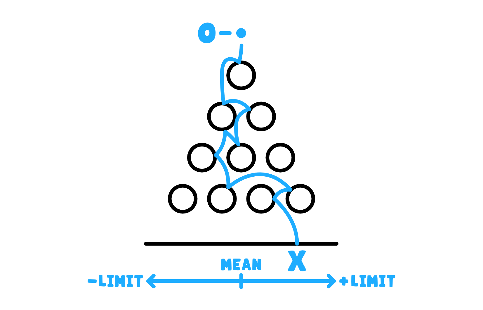
The above video shows a simulation of a quincunx toy also known as the Galton board. It’s a statistical toy created by Sir Francis Galton that provides a nice visual demonstration of the Central Limit Theorem - that theorem explaining how the distribution of the sampling mean is normal regardless of the shape of the distribution that the samples are coming from. It’s a very standard result in introductory statistics and this toy nicely, in real time, demonstrates its emergence.

However, there is an alternative view we can take on why the normal distribution appears out of apparent chaos at the base of the quincunx. This view is still statistical in nature but the idea behind it relies much more on nature than just pure statistics. In nature, everything tends toward chaos, entropy increases, things get progressively more disorderly until they reach a state of maximal entropy. So nature longs for unpredictability. How can we then explain the emergence of the normal distribution inside the quincunx? Wouldn’t nature, in this case gravity, want the balls to be equally distributed among all the bins at the bottom of the board to maximize each ball’s unpredictability? The answer is no and this post (hopefully intuitively) explains why that’s the case and why in fact the normal distribution maximizes entropy under the conditions implied not only by the quincunx but also by the Central Limit Theorem in general.

---

The Rules of Quincunx

The quincunx was a toy imagined by Sir Francis Galton based on the following set of assumptions:

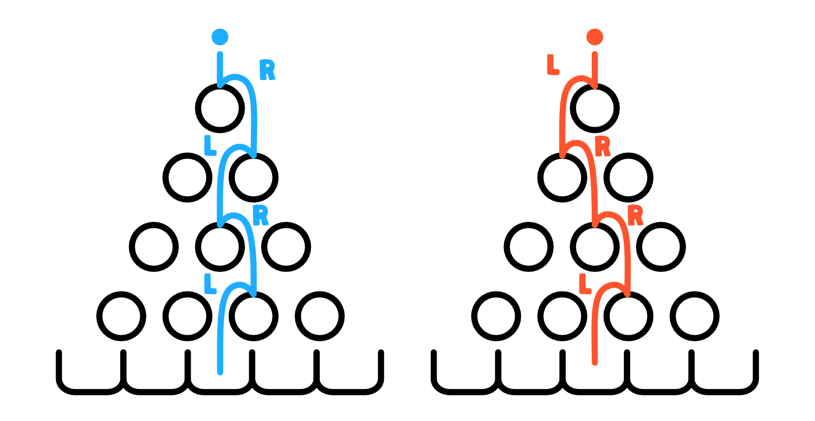
• the board is filled with obstacles arranged in a quincunx pattern - that’s the pattern of dots for number 5 on a regular die ⁙
• at the bottom of the board there are small equally spaced compartments for the balls to fall into
• at the top, balls are thrown in one-by-one, right above the central obstacle
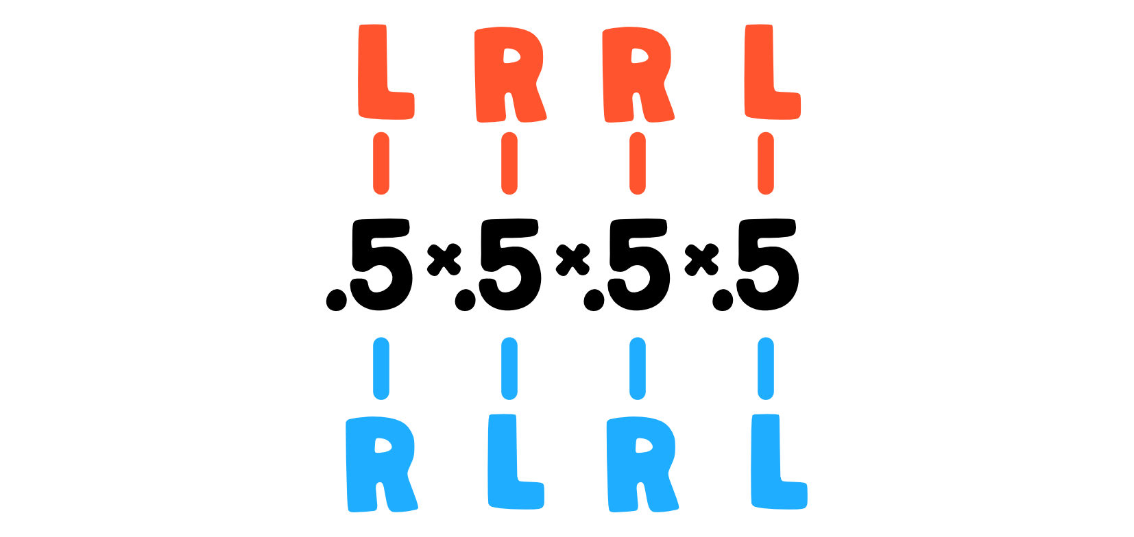
• as the balls fall through the grid, they encounter one obstacle at each level and at every encounter they have a 50-50 chance of going left (L) or right (R) - so each encounter is essentially a coin toss with probability $p=0.5$
• the compartment in which a ball lands depends on the sequence of coin tosses the ball makes at each encountered obstacle
• so if the depth of the board is $d$, the ball’s compartment is determined by the number of successes (R moves) in $d$ coin tosses (obstacle encounters) - that is if $d=4$ and two balls take paths RLRL and LRRL, they will both end up in the same compartment because out of 4 coin tosses (obstacle encounters) they got 2 heads (R)
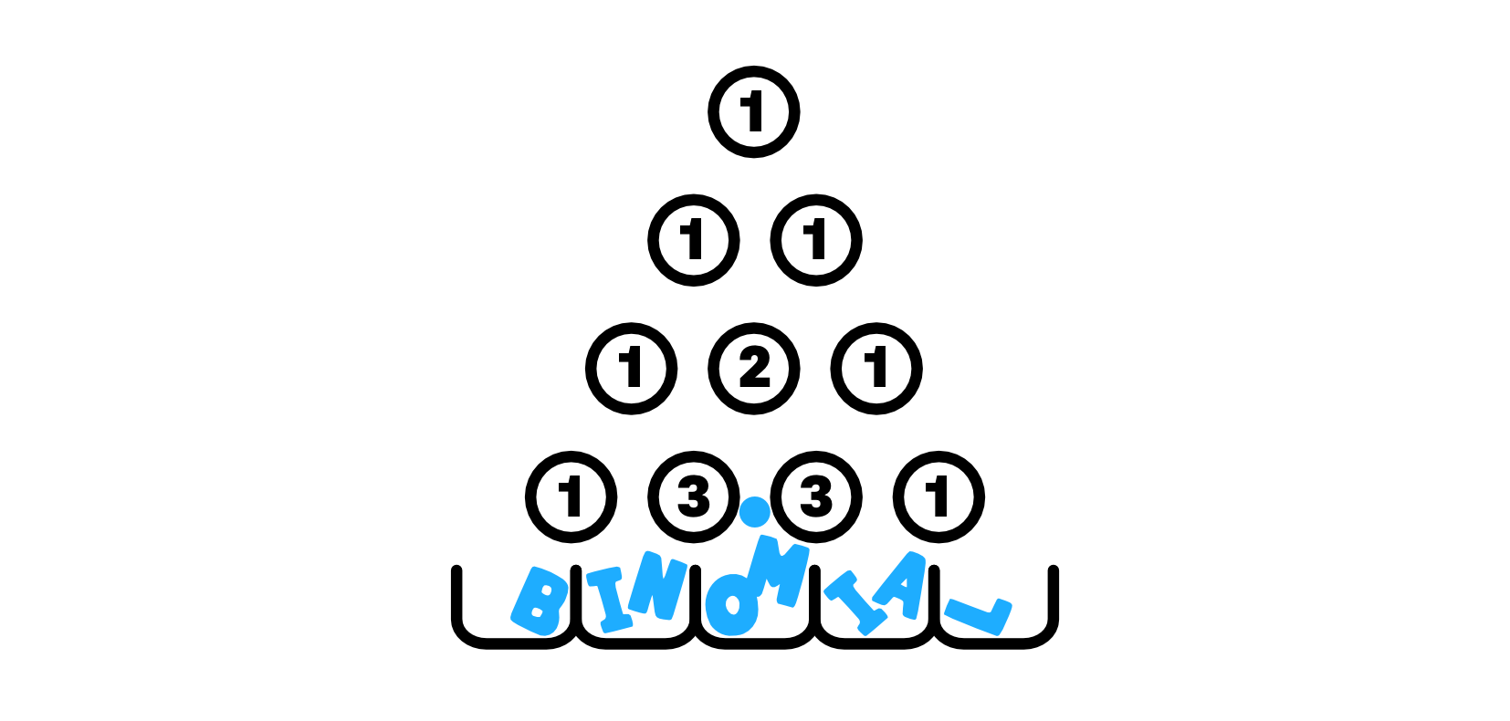
• so the the ball’s final resting place is in fact a binomial random variable - a random variable defined by the number of successful coin tosses $k$ in $d$ total coin tosses

Now that we know that the ball’s destined compartment follows a Binomial distribution, we can look at the probability of ending in any of the compartments. The probability of a binomial random variable taking on a certain value depends solely on the number of successes $k$ in $d$ trials. This is what we have already established by noting that the trajectories RLRL and LRRL lead to the same compartment if the depth of the board is $d=4$. Thus the probability of ending in a certain compartment is just the sum of probabilities of all $d$-long sequences with exactly $k$ successes - since each such sequence leads the ball to the same compartment. How many such sequences there are is given by the handy $d$ choose $k$ formula:

\[{d \choose k} = \frac{d!}{k!(d-k)!}.\]

And because our coin tosses are fair, the probability of a specific $d$-long sequence is exactly the same as any other $d$-long sequence, namely $0.5^d$. Thus the preference of one compartment over another lies solely in the binomial coefficient ${d \choose k}$.

So what manifests itself at the bottom of a theoretical Galton board is in fact a binomial distribution, not the normal one. It is just a nice coincidence that the discrete binomial distribution very much resembles its normal continuous counterpart, even when the number of trials $d$ is small. But as the number of trials $d$ grows it can actually be shown with the De Moivre-Laplace theorem that the binomial distribution approaches the normal one - a special case of the Central Limit Theorem (CLT). So throwing many balls into a deep enough theoretical Galton board does give quite a beautiful physical example of the CLT in practice.

There’s a catch though…

But there’s a catch. I deliberately kept saying theoretical Galton board because the behavior I described above is indeed purely theoretical. In the actual Galton board (or a close physical simulation of it) the balls don’t actually toss a coin each time they encounter an obstacle. They fall through the board according to the rules of physics, guided by gravity, bouncing, sliding and interacting with the obstacles and each other in a much richer way than a fifty-fifty flip of a coin. Yet, both the simulations and the real physical toys seem to produce the approximately normal distribution at their base. Why?

I think there are two plausible explanations for this. First, it might be that all the bouncing, sliding and hoping just cancels out and the theoretical rules of statistics prevail. This is entirely possible but very hard to test. Thus I think there’s a better explanation, one that allows nature to do all its randomness yet still permits us to carry out our statistical analysis of what we can expect on average. This view relies on the fundamental concept of entropy which just assumes that nature tends towards maximum unpredictability. As we will see in a bit, the normal distribution actually achieves the nature’s goal… and the math is even more joyful than the binomial explanation!

I have of course not come up with this explanation myself. It comes from a somewhat mysterious paragraph on the Galton Board’s Wikipedia entry. I honestly don’t think it belongs there, as it’s not very well explained and thus doesn’t fit the encyclopedic mission of Wikipedia, but it nevertheless provided several joyous hours of trying to figure out what the author meant. So if you are now enjoying this blog post, the thanks goes to that mysterious author of that mysterious paragraph.

Entropy

So what’s entropy? Entropy is a concept borrowed from physics and made the cornerstone of modern information theory. In physics, entropy is kind of a watchdog that allows certain processes while forbidding others. Your mug can break on its own but it will never unbreak back into itself. This is because of entropy. The entropy of a broken mug is much higher than that of an unbroken one. In essence, there are millions of ways a specific mug can break but there was only one way in which it wasn’t broken. So for an isolated system¹, a mug in this case, the nature only allows entropy to increase, never decrease.

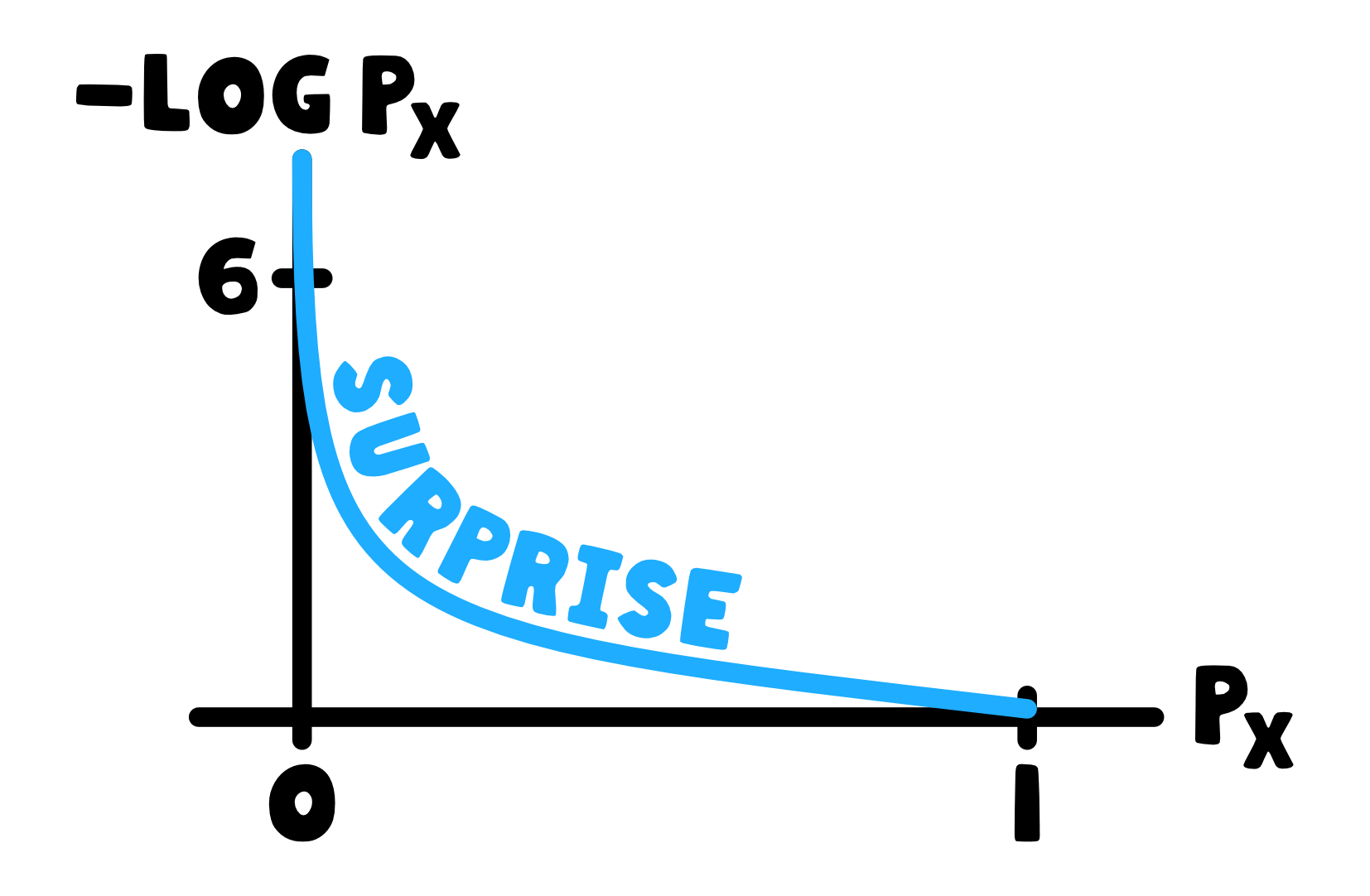
Information theory borrowed this concept and applied it in its own but similar way to the study of random variables. For a random variable $X$ defined by its probability function $p(x)$ the entropy quantifies how much surprise the random variable carries. If $X_1$ is a toss of a coin and $X_2$ is a roll of a die, the entropy of the roll is more than that of a toss: $H(X_2) > H(X_1)$. This is because each roll of a die is more unpredictable, generates more surprise, than each toss of a coin. The die has 6 equally likely options while the coin only has 2. The surprise value of each outcome, a specific number on a die or a side of a coin, is measured by $-1$ times the logarithm of its probability, $\log p(x)$. The base of the logarithm doesn’t matter, what matters is that the closer the probability $p(x)$ is to 1, the closer the $-\log p(x)$ is to 0. Just as we would want, since a very likely event doesn’t generate much surprise. Conversely as the probability tends toward 0, $-\log p(x)$ tends toward infinity. Again a desirable outcome since the more unlikely an event is, the more surprised we would be if it actually happened.

With this logarithmic measure of surprise we can quantify the entropy of the entire distribution $p(x)$. For a discrete distribution, like that of a coin flip, roll of a die or the ball’s theoretical position at the base of the quincunx , the entropy $H(X)$ is defined by the sum:

\[H(X) = -\sum_{x \in \mathcal{X}}p(x)\log p(x),\]

where the sum is taken over all possible values of $x$. $\mathcal{X} = \lbrace\text{heads},\text{tails}\rbrace$ for a coin, $\mathcal{X} = \lbrace 1, 2, 3, 4, 5, 6 \rbrace$ for a die. This definition just takes the surprise value of each outcome and multiplies it by the probability of that outcome actually happening, then sums it up over all possible outcomes. Very straightforward.

Extending this to continuous distributions, like the normal one, we just replace the summation with an integral to get:

\[-\int_{-\infty}^{\infty}f(x)\log f(x)dx.\]

This is in essence the same as the sum, we have just shrunk the step size to infinitesimally small step $dx$ and extended the range to cover the entire real line from minus infinity to infinity - the most general support for a continuous random variable. We have also replaced $p(x)$ with $f(x)$ to make the distinction between the discrete and the continuous case.

Nature maximizes entropy

As we said before, nature maximizes entropy. Things stir, break, become more disorderly if left to their own devices. Nature just prefers the highest possible degree of chaos available to it. It’s just an irrefutable fact. But we can use it to our own advantage. When we observe some data, in our case the data about how many balls end up in each compartment of the quincunx, we can ask ourselves:

Given the data I see, what’s the most likely generating distribution that this data is coming from?

There are several ways one can define most likely. Frequentist would tell you it’s defined by the maximum likelihood function. Bayesians would argue you need to combine the maximum likelihood with your prior convictions. Information theorists say: well, nature wants chaos, so the most likely generating distribution is the one with the highest entropy. I like that idea because its fully grounded in what nature does not what monkeys want it to do. So given some data that implies certain constraints on the group of plausible data-generating distributions, we should pick the one with the highest entropy. This is called the Principle of maximum entropy.

Maximum entropy inside the quincunx

So what distribution maximizes the entropy inside the quincunx? To figure this out, we can first represent each ball a little more true to its nature than the binomial random variable does. We can think of each ball as a continuous one dimensional random variable $X$ that falls into the board at some position we denote as 0 and ends its journey through the board at some new position $x$. The probability of landing at any $x$ at the base of the quincunx is denoted with $f(x)$. We don’t know at what $x$ it will end up but we know there are only so many bounces it can make after which it has to come to rest. We also know that because there are only so many obstacles and the depth $d$ of the board is finite, there’s a physical limit on how far off its starting position the ball can fall. This representation of each ball has thus some fixed unknown average ending position $\mu$ and also some fixed unknown variance $\sigma^2$. The variance is fixed because the board’s height is finite and so the ball can only wander off to the sides by a certain fixed amount. And because of this the average position is also fixed, since there will be some average landing position of the ball between the left and right limit imposed by the fixed variance.

So that’s our new representation of the ball. Hopefully you can appreciate that this is much closer to what actually happens with the ball inside the quincunx than the coin-flip-obstacle alternative. Now nature asks:

I want to maximize entropy (unpredictability) but this random ball has some fixed mean and fixed variance in its landing position. So among all the distributions with a given mean and variance, which is the one that maximizes entropy?

In other words, if we know that there are constraints on the mean and variance, what distribution should nature choose such that the entropy of the random variable represented by the ball is maximized?

The promised joyful math

This is a constrained maximization problem and since we have a good working definition of our random ball and also its entropy function we can attack it with the method of Lagrange multipliers. First, without the Lagrange multipliers, the constrained maximization can be defined as:

\[\begin{align*} \max_{f} \quad & \mathcal{L}(f) = -\int_{-\infty}^{\infty} f(x) \ln f(x) \, dx \\ \text{s.t.} \quad & \int_{-\infty}^{\infty} f(x) \, dx = 1, \\ & \int_{-\infty}^{\infty} f(x)x \, dx = \mu, \\ & \int_{-\infty}^{\infty} f(x)(x-\mu)^2 \, dx = \sigma^2. \end{align*}\]

Our main equation $\mathcal{L}(f)$ is the entropy function with $e$ taken as the base of the logarithm. The constraints are that all the probabilities must integrate to 1 (otherwise it’s not a valid probability distribution), the mean has to be equal to $\mu$ and the variance must be equal to $\sigma^2$ - the two constraints implied by the toy’s design. To solve this with a pen and paper, we can transform the above set of equations into a single one with the help of Lagrange multipliers:

\[\begin{align*} \mathcal{L}(f) = & -\int_{-\infty}^{\infty} f(x) \ln f(x) \, dx \\ & + \lambda_0 \left( \int_{-\infty}^{\infty} f(x) \, dx - 1 \right) \\ & + \lambda_1 \left( \int_{-\infty}^{\infty} f(x)x \, dx - \mu \right) \\ & + \lambda_2 \left( \int_{-\infty}^{\infty} f(x)(x-\mu)^2 \, dx - \sigma^2 \right). \end{align*}\]

The idea behind Lagrange multipliers is simple. We want to maximize $\mathcal{L}(f)$ with some constraints thrown in. If we had no constraints we would take the derivative of $\mathcal{L}(f)$ with respect to $f$, set it equal to 0 and solve for $f$. After checking that the second derivative is negative, we would certify that the $f$ we have found is indeed the function that maximizes $\mathcal{L}(f)$. Nice, but that only works when we don’t have any constraints. So what if we do? Well, Lagrange multipliers transform a constrained maximization problem of multiple equations into a problem of a single unconstrained equation - and we know how to solve that. They do it by tagging on penalization terms to the main equation. These penalization terms are just the constraints written such that if they aren’t satisfied, our maximization suffers. And if they are satisfied, all the penalization terms equal 0 and the problem reverts to the original main equation. That’s hopefully an intuitive explanation of Lagrange multipliers - I would check this example from Wiki if you want more intuition.

Armed with the Lagrange-ized equation, we can proceed to maximize it by the usual method. Find the derivative, set it to 0, check that the 2nd derivative is negative and solve the first derivative in terms of $f$. Before we do that though, we can see that we don’t really need the 2nd Lagrange multiplier. The constraint for $\mu$ is implicitly included in the constraint for the variance and so we can drop it and make our life a little simpler. The Lagrangian that we will thus be solving is:

\[\begin{align*} \mathcal{L}(f) = & -\int_{-\infty}^{\infty} f(x) \ln f(x) \, dx \\ & + \lambda_0 \left( \int_{-\infty}^{\infty} f(x) \, dx - 1 \right) \\ & + \lambda_1 \left( \int_{-\infty}^{\infty} f(x)(x-\mu)^2 \, dx - \sigma^2 \right). \end{align*}\]

Taking the derivative with respect to $f$ yields:

\[\begin{align*} \frac{d\mathcal{L}}{df(x)} = & -\left(1\cdot\ln f(x) + f(x)\cdot\frac{1}{f(x)}\right) \\ & + \lambda_0(1 - 0) \\ & + \lambda_1\left(1\cdot(x - \mu)^2 - 0\right). \end{align*}\]

To solve for $f(x)$ we just let this equal to 0 (maximum occurs where the function’s derivative is 0) and rearrange the terms:

\[\begin{align*} 0 = & -\ln f(x) - 1 + \lambda_0 + \lambda_1(x - \mu)^2 \\ \ln f(x) = & - 1 + \lambda_0 + \lambda_1(x - \mu)^2 \\ f(x) = & \, e^{- 1 + \lambda_0 + \lambda_1(x - \mu)^2} \end{align*}\]

This is a general solution for $f(x)$ and we know it’s the one that maximizes our entropy loss function $\mathcal{L}$, because the second derivative is negative

\[\frac{d^2\mathcal{L}}{d^2f(x)} = -\frac{1}{f(x)}.\]

So to get our specific distribution, we now just need to plug our general solution back into our constraints and solve for $\lambda_0$ and $\lambda_1$. First, let’s make sure that the integral evaluates to 1 making $f(x)$ a valid probability distribution function:

\[\begin{align*} 1 = & \int_{-\infty}^{\infty} f(x) \, dx \\ 1 = & \int_{-\infty}^{\infty} e^{- 1 + \lambda_0 + \lambda_1(x - \mu)^2}\, dx \\ 1 = & \int_{-\infty}^{\infty} e^{- 1 + \lambda_0}\cdot e^{\lambda_1(x - \mu)^2}\, dx \\ 1 = & \,e^{- 1 + \lambda_0} \int_{-\infty}^{\infty} e^{\lambda_1(x - \mu)^2}\, dx \\ e^{1 - \lambda_0} = & \int_{-\infty}^{\infty} e^{\lambda_1(x - \mu)^2}\, dx \end{align*}\]

At this point we need to integrate the right hand side but that’s no easy job. However, if $\lambda_1$ would be negative than it would really resemble a Gaussian Integral for which we could use the result $\int_{-\infty}^{\infty} e^{-a(x+b)^2}\, dx = \sqrt{\pi/a}$. So can we assume that the Lagrange multiplier $\lambda_1$ is actually negative? From our results thus far we can see that if $\lambda_1$ is positive, than this integral diverges to infinity which would produce a positive penalty in our original Lagrangian function. This is not what we want since our original Lagrangian is a maximization problem and thus the penalty should be in the negative direction. Therefore we can safely assume that $\lambda_1$ can only attain negative values. Since this is the case, the above integral becomes a Gaussian integral and we can solve it by the well established result $\int_{-\infty}^{\infty} e^{-a(x+b)^2}\, dx = \sqrt{\pi/a}$ (3b1b has a great video explaining how $\pi$ appears here seemingly out of nowhere and how integrals of this type are solved). Using this result we get:

\[\begin{align*} e^{1 - \lambda_0} = & \int_{-\infty}^{\infty} e^{\lambda_1(x - \mu)^2}\, dx \\ e^{1 - \lambda_0} = & \sqrt{\frac{\pi}{-\lambda_1}} \\ e^{- 1 + \lambda_0 } = & \sqrt{\frac{-\lambda_1}{\pi}}. \end{align*}\]

So in order to satisfy the first constraint, this relationship between $\lambda_0$ and $\lambda_1$ must hold true. We will come back to this result once we derive more knowledge about this relationship from the second constraint. To satisfy the second constraint, we follow a similar set of steps and use all the results we got so far:

\[\begin{align*} \sigma^2 = & \int_{-\infty}^{\infty} f(x)(x-\mu)^2 \, dx \\ \sigma^2 = & \int_{-\infty}^{\infty} e^{- 1 + \lambda_0 + \lambda_1(x - \mu)^2}(x-\mu)^2 \, dx \\ \sigma^2 = & \int_{-\infty}^{\infty} e^{- 1 + \lambda_0} e^{\lambda_1(x - \mu)^2}(x-\mu)^2 \, dx \\ \sigma^2 = & e^{- 1 + \lambda_0}\int_{-\infty}^{\infty} e^{\lambda_1(x - \mu)^2}(x-\mu)^2 \, dx \\ \sigma^2 = & \sqrt{\frac{-\lambda_1}{\pi}}\int_{-\infty}^{\infty} e^{\lambda_1(x - \mu)^2}(x-\mu)^2 \, dx \\ \end{align*}\]

At this point, we can perform a substitution to simplify the solving of the right-hand side. Substituting $x-\mu = y$ and $dx = dy$ we get:

\[\begin{align*} \sigma^2 = & \sqrt{\frac{-\lambda_1}{\pi}}\int_{-\infty}^{\infty} e^{\lambda_1y^2}y^2 \, dy \\ \end{align*}\]

This is another tough integral to crack but we can use another established results that generalizes the Gaussian Integral we used before. The result we’ll use is this:

\[\begin{align*} \int_{-\infty}^{\infty} x^{2n}e^{-ax^2} \, dx = & \frac{2(2n - 1)!!}{a^n2^{n+1}}\sqrt{\frac{\pi}{a}} \end{align*}\]

Here the double factorial ($!!$) stands for the factorial where we only take all the odd or all the even numbers into account - depending on whether the number we want the double factorial of is even or odd. The case that fits our equation is the case when $n=1$ since then the left-hand side becomes $x^2e^{-ax^2}$. And the right-hand side evaluates to:

\[\begin{align*} \int_{-\infty}^{\infty} x^{2}e^{-ax^2} \, dx = & \frac{2(2n - 1)!!}{a^n2^{n+1}}\sqrt{\frac{\pi}{a}} \\ = & \frac{2(2 - 1)!!}{a^12^{1+1}}\sqrt{\frac{\pi}{a}} \\ = & \frac{2}{4a}\sqrt{\frac{\pi}{a}} \\ = & \frac{1}{2}a^{-1}a^{-1/2}\sqrt{\pi} \\ = & \frac{1}{2}a^{-3/2}\sqrt{\pi} \\ = & \frac{1}{2}\sqrt{\frac{\pi}{a^3}} \end{align*}\]

Plugging in $-\lambda_1$ instead of $a$ and putting it back into the result we obtained from solving the second constraint, we finally get to:

\[\begin{align*} \sigma^2 = & \sqrt{\frac{-\lambda_1}{\pi}}\int_{-\infty}^{\infty} e^{\lambda_1y^2}y^2 \, dy \\ \sigma^2 = & \sqrt{\frac{-\lambda_1}{\pi}}\frac{1}{2}\sqrt{\frac{\pi}{-\lambda_1^3}} \\ \sigma^2 = & \frac{1}{2}(-\lambda_1)^{1/2}(-\lambda_1)^{-3/2}\pi^{-1/2}\pi^{1/2} \\ \sigma^2 = & \frac{1}{2}(-\lambda_1)^{-1} \\ \sigma^2 = & \frac{1}{-2\lambda_1} \\ \lambda_1 = & \frac{1}{-2\sigma^2} \end{align*}\]

Nice! So now we have a general expression for the second Lagrange multiplier in terms of our fixed variance $\sigma^2$. Using this result, we can plug it back into the relationship between $\lambda_0$ and $\lambda_1$ we obtained from solving the first constraint:

\[\begin{align*} e^{- 1 + \lambda_0 } = & \sqrt{\frac{-\lambda_1}{\pi}} \\ e^{- 1 + \lambda_0 } = & \sqrt{\frac{-\left(\frac{1}{-2\sigma^2}\right)}{\pi}} \\ e^{- 1 + \lambda_0 } = & \frac{1}{\sqrt{2\pi\sigma^2}} \end{align*}\]

And with this, we can conclude the maximization by taking the general form of the function $f(x)$ that we derived at the very beginning and plugging in all the results we obtained along the way:

\[\begin{align*} f(x) = & e^{- 1 + \lambda_0 + \lambda_1(x - \mu)^2} \\ = & e^{- 1 + \lambda_0} e^{\lambda_1(x - \mu)^2} \\ = & \frac{1}{\sqrt{2\pi\sigma^2}} e^{\lambda_1(x - \mu)^2} \\ = & \frac{1}{\sqrt{2\pi\sigma^2}} e^{-\frac{(x - \mu)^2}{2\sigma^2}} \end{align*}\]

And, just like that, we have our result! …okay, I admit it wasn’t, just like that, but if you got this far, I assume you extracted some joy from this somewhat tedious process of maximizing the Lagrangian. We had to use established results to solve some of the integrals along the way, which I can understand might be a bit frustrating, but this post would be way too dense if we were to derive the Gaussian integrals from scratch. And we still did a hefty dose of derivatives and actual pen-&-paper mathematics nonetheless. The main point though, is that under the assumptions of the fixed mean and variance of the ball’s final resting position, we can expect the distribution of the positions to be normal because this is the distribution that maximizes nature’s ultimate desire - the entropy. And if you ask me, that’s one beautiful result.

And what about the Central Limit Theorem?

So can we generalize this result beyond the walls of the quincunx? If you look at the wiki page of the Central Limit Theorem you’ll find at least 4 different definitions for the CLT. But what all of them have in common is that for the CLT to emerge from random sampling, the mean and variance of the underlying distribution must be finite! These are exactly the two constraints that lead us to the normal distribution in the process of maximizing entropy. So the CLT is not just a purely frequentist result but also a natural consequence of nature’s desire for disorder and chaos.

Sources

• Similar derivation by Joshua Goings
• And one more by Sam Finlayson
• Galton’s book where he proposes the quincunx toy (p.70)
• Rigorous information theoretic proof of CLT

1. Isolated just means that we are not adding in any external work, in the physics sense, to the system. We can reduce broken mug’s entropy by fixing it with some glue but it will never fix itself ↩